Scanstation: The Perfect Stitch

A perfectly built machine scanning a perfectly consistent slab produces a perfect stitch and perfect measurements. The math inside Scanstation is deterministic, so when a stitch is off, it is not noise and it is not luck: it is a measurement of some real, physical deviation in the machine or the slab. The cost is bounded and specific: inaccurate stitching produces measurable inaccuracies in Y dimensions and locations, while X remains correct provided the machine’s travel is consistent. This guide shows how to find the deviation, with a straightedge, a tape measure, and a little patience.

Why “perfect” is even on the table

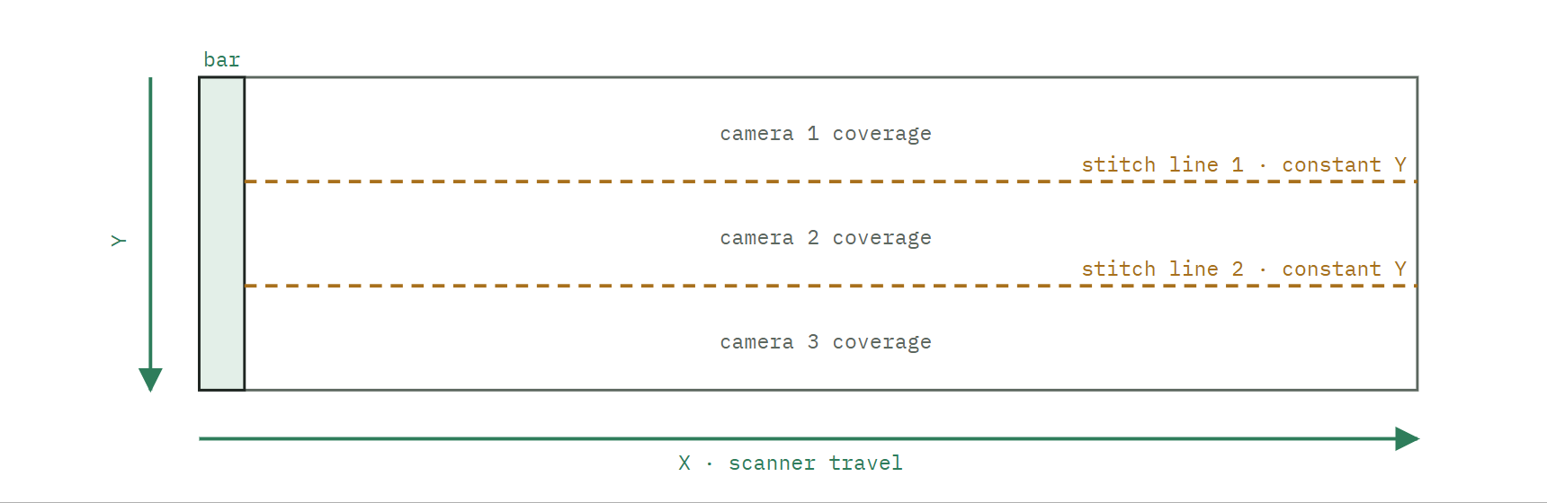
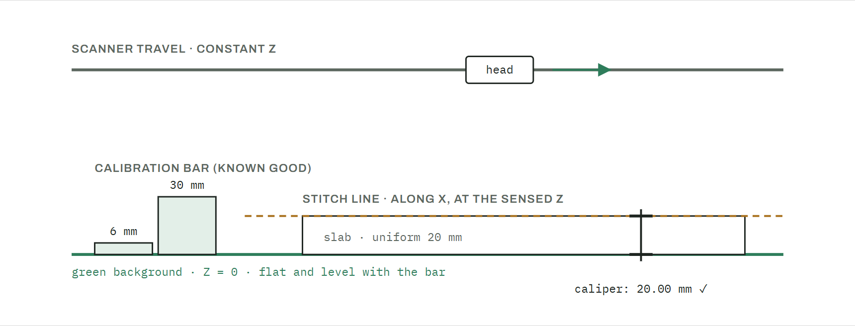
Scanstation covers the slab with multiple cameras in a single pass. Adjacent cameras are joined along a stitch line: a line of constant Y, set at the midpoint between each camera pair, running the full length of the machine along X at the defined (or sensed) height. A machine with n cameras has n − 1 stitch lines. A three-camera machine has two. To join two cameras correctly along such a line, the software needs exactly one physical fact: the true height of the slab surface along that line. Everything else is geometry it already knows.

That single fact rests on a short chain of physical assumptions:

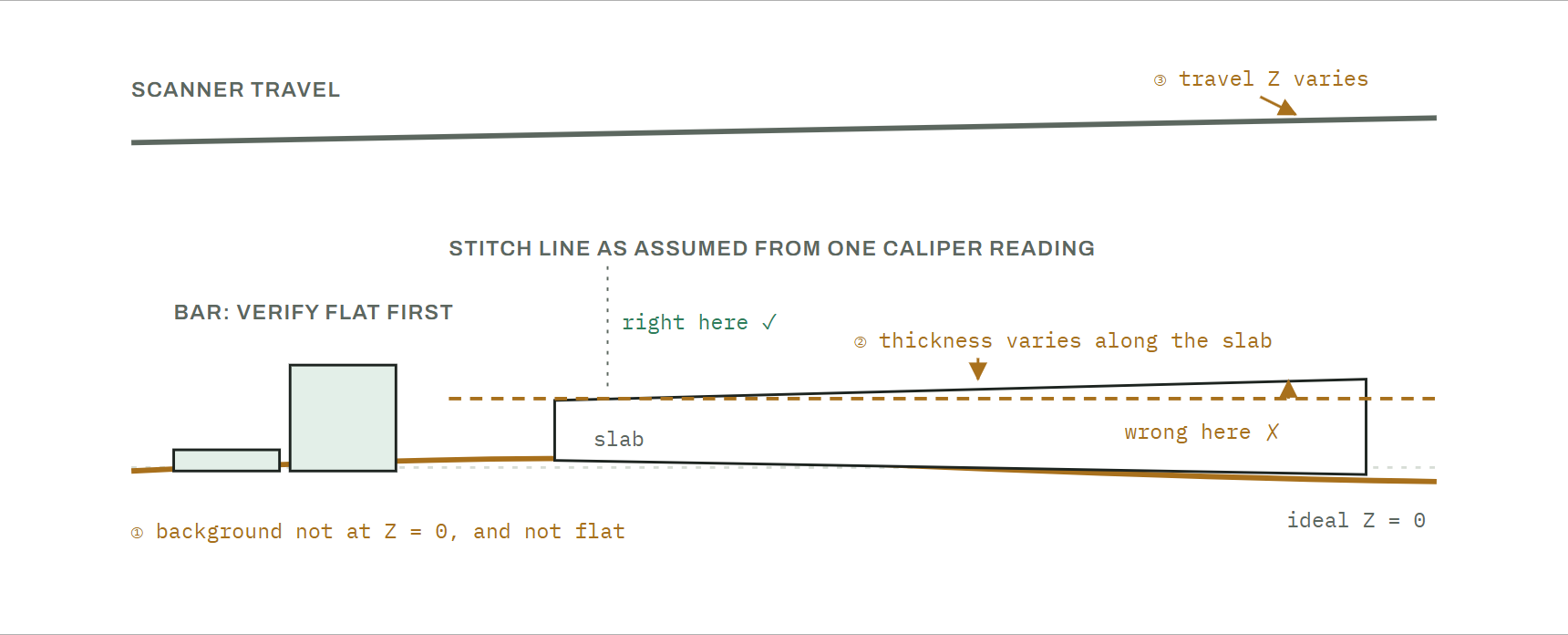
The background the slab lies on sits at height zero: flat, and level with the calibration reference.
The slab has one thickness, so a caliper reading anywhere is a reading everywhere.
The scanner head travels at constant height.
The calibration bar, the machined reference that defines 6 mm and 30 mm for the whole system, is mounted without a bend.

When all four hold, thickness at the stitch line is surface height, the math closes exactly, and the stitch is perfect. When any one of them doesn’t hold, the stitch inherits the difference, millimeter for millimeter. That is the entire story of stitch anomalies, and it is good news: each assumption can be checked independently, with ordinary shop tools, and each failure has a known compensation.

Plan view of a three-camera machine: three camera coverage bands span the field across Y, joined at two dashed stitch lines of constant Y that run the full length of the machine along X, the scanner travel direction. The calibration bar sits along one edge. — **The stitch lines, seen from above** (three-camera machine shown). Each line lies at the constant Y midpoint between a camera pair and runs the full length of travel along X, from the calibration bar to the far end. The cross-sections that follow are cut along one of these lines, which is why the stitch line appears in them as a horizontal line at the slab surface, not a vertical cut.

Cross-section of an ideal machine, cut along a stitch line: flat background at Z equals zero, calibration bar with 6 and 30 millimeter planes, scanner head traveling at constant height, and a uniform slab. The stitch line runs horizontally along X at the sensed height, coinciding with the slab surface, and one caliper reading anywhere on it gives the height everywhere. — **The ideal machine**, cut along a stitch line. Background at exactly Z = 0, uniform slab, level head travel. The stitch line coincides with the slab surface at one constant height along its whole length, so a single caliper reading, taken anywhere on the line, gives the surface height everywhere on it, and the stitch closes perfectly with no adjustment.

The same cross-section with exaggerated real-world deviations: the background bows away from Z equals zero, the slab thickness varies along its length, and the scanner travel is not perfectly level. A dashed line shows the single height a caliper reading assumes for the whole stitch line, matching the real surface at the measurement point but diverging from it where the thickness differs. — **Where reality enters** (deviations exaggerated). Every installed machine sits somewhere between this picture and the ideal one. A single caliper reading still fixes one height for the entire stitch line: correct at the point of measurement, off everywhere the slab or background differs, by exactly the amount of the difference. Each numbered deviation is independent, and the job of diagnosis is to measure them one at a time.

Proving where the deviation lives

Every diagnosis starts from the one component we can trust unconditionally: the calibration bar. It is precision-machined; its two planes define 6 mm and 30 mm for the entire system. The only thing that can go wrong with it is mounting, so the first check is a full-length straightedge along the bar. If the straightedge shows no bend, the bar is your reference plane, full stop.

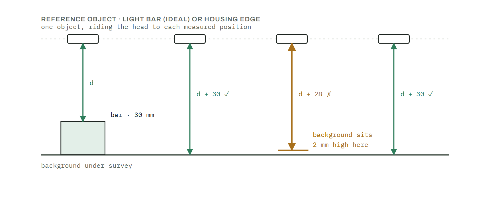
From there, the scan head itself becomes a measuring bridge. The ideal reference to measure from is the light bars; if you’d rather not open the scan head, the edge of the housing works just as well. Either way it is a fixed reference object riding the head, sitting close to the calibration bar, which makes the distance from reference to bar easy to measure at several points, and nothing in what follows changes with the choice. (If the lights turn out not to be perfectly parallel to the bar, the photometric effect is real but small, almost certainly below anything a customer would notice. Their diagnostic value is what matters here.)

Now the decisive measurement: from the same reference object, measure down to the background at many points across the whole field. Since the bar’s top plane stands 30 mm above a true Z = 0 background, every one of those measurements should equal the reference-to-bar distance plus exactly 30 mm, everywhere. Any point where it doesn’t is a point where the background deviates from zero, and the amount of the miss is the amount of the deviation. This isn’t an estimate; it is a direct survey of the surface the entire system stands on.

Survey method: one reference object on the scan head (the light bar, or the housing edge) rides the head along X and is shown at four positions. At each position, measure down: to the calibration bar to get distance d, then to the background across the field. Each background measurement should equal d plus 30 millimeters; one highlighted point measures short, revealing where the background sits above zero. — **The 30 mm test.** One fixed reference object on the scan head rides the head to each position shown. The light bar is ideal, and the housing edge works without opening the head; the conclusions are identical. At every stop, reference-to-background must equal reference-to-bar + 30 mm, at *every* point across the field. Each miss is a direct, local measurement of how far the background sits from Z = 0: no software involved, no interpretation required.

Everything flows from one question: are there Z sensors?

Z sensors read the actual slab surface at the stitch line, at scan time. That single capability splits the whole analysis in two, because it decides whether the system measures reality or must assume it.

Branch 1: Z sensors at the stitch line

STITCH LINE
The sensor reads the real surface, so the stitch is guaranteed to the precision of the sensor. In practice, any residual is at the millimeter scale, comfortably inside the layout tolerances the vast majority of shops hold. Background deviation and slab variation are both compensated automatically.

REPORTED THICKNESS
The sensor measures height above the background as calibrated. Calibrate against an empty background and every point should read 0; whatever it reads instead is a Z map of the build. Deviation from zero is technically wrong but well compensated, given good repeatability. The cost shows up elsewhere: if the map reads, say, −2 mm everywhere, stitches stay perfect while every reported slab thickness is off by that same 2 mm.

SENSOR PRECISION
An inaccurate or drifting sensor passes its error straight into the stitch. If stitch residuals exceed the sensor’s rated precision, suspect the sensor or its mounting before anything else.

Branch 2: No Z sensor (caliper-entered thickness)

FLAT BACKGROUND AND UNIFORM SLAB
The ideal case genuinely works: one caliper measurement at the stitch line gives a perfect stitch. This is the configuration the caliper workflow was designed for.

ONE DEVIATION
If the background is off zero but the slab is flat, a correct caliper reading will register as a wrong stitch. The error is the background’s, not the measurement’s. Once the 30 mm survey has mapped the offset, it can be corrected with a known adjustment. Likewise a wedged slab on a true background: measure at the stitch line itself, not at the slab edge.

BACKGROUND OFF AND SLAB NOT FLAT
Two unknowns, one measurement, no sensor: the system cannot separate them, and neither can an operator. Even manual stitch adjustment is chasing a moving target, and no guarantee can be made. This is the one configuration with no compensation, and the honest fix is to remove one of the unknowns: level the background, or add Z sensors.

The tape test: seeing deviations without measuring anything

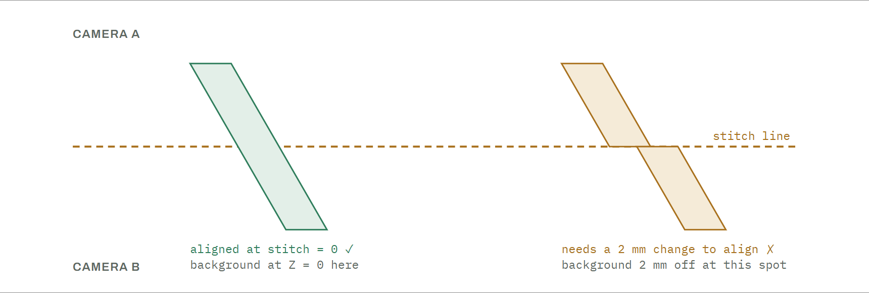
Before reaching for a tape measure at all, there is a purely visual check: place diagonal strips of tape across a stitch line (on the bare background, on a slab, or both) and see whether they render the way they should. The diagonal is what makes it work: a stitch error displaces the two halves of the image across the seam, so a strip crossing square to the line just slides along its own length and hides the shift. A diagonal edge turns the same displacement into a sideways jog you can’t miss.

On the bare background, manually set the stitch to 0. If the background truly sits at Z = 0 where the strip crosses, the tape lines up with no discontinuity. If you have to dial the stitch to + or − some millimeters before it aligns, the background is off from the calibration bar by exactly that much, at that spot. The adjustment dial has become your measuring instrument.

Now lay several strips along the same stitch line. If the strip on the left aligns at 0 but the strip on the right needs an adjustment, the background does not hold a consistent Z left to right on the stitch line. You have localized variation without taking a single measurement. Each strip is one survey point; several strips are the deviation map of the seam. The same test runs on a slab: set the stitch to the caliper thickness and the strips report whether the surface at the seam matches it. On a machine with Z sensors, the strips should align with no manual adjustment at all, so any adjustment they need is a direct read of sensor error.

The test’s one limitation is where it can look: only the stitch line itself. A strip placed anywhere else crosses no seam and has nothing to reveal, so the rest of the field remains the territory of the measured survey described above.

Top view of a stitch line with two diagonal tape strips crossing it. The left strip crosses without discontinuity, showing the background at zero at that spot. The right strip jogs sideways at the seam and needs a two millimeter stitch change, in either direction, to align, showing the background is two millimeters off at that spot. — **The tape test on a bare background**, stitch manually set to 0, seen from above. The left strip crosses the seam cleanly; the background is at Z = 0 there. The right strip jogs, and the stitch adjustment needed to close the jog is the background’s deviation at that spot. Different strips needing different adjustments means the background’s Z varies along the stitch line itself.

Walking the chain, in order

The order matters: each step certifies the reference the next step leans on. It is tedious, and that is the point. At the end, the deviation has a location and a number, not a vibe.

Certify the calibration bar. Lay a full-length straightedge along the bar. No bend means the bar is your reference plane. (A bent bar corrupts everything downstream. Remount before measuring anything else.)
Tie a reference object to the bar. Pick a fixed reference on the scan head. The light bar is the ideal spot, and the edge of the housing serves if you’d rather not open the head. Measure reference-to-bar at several points along the bar, recording the distance d at each. This makes the reference object a portable extension of the reference plane.
Survey the background: the 30 mm test. From the same reference object, measure down to the background at many points across the whole field. Every reading should be d + 30 mm. Log each miss with its position: this is your background deviation map, and it is the single most informative artifact in the whole diagnosis. (The tape test above produces the same map visually, strip by strip, and is a fine place to start before measuring.)
If Z sensors are fitted: calibrate on the empty background. Every point should read 0. The pattern of what it reads instead tells you two things at once: varying readings confirm the survey from step 3, and a uniform offset predicts exactly how far reported slab thickness will be biased.
Characterize the slab. Caliper the slab at several points, including directly on the stitch line. Stone is a natural product, and its thickness can change measurably across a slab. Knowing that it does is what separates a machine problem from a material fact.
Read the result off the branch table. With the bar certified, the background mapped, and the slab characterized, the branch diagram above assigns the anomaly to its cause, and the table below gives the consequence and the fix.

What each deviation costs, and what fixes it

Deviation	With Z sensors	Without Z sensors	Compensation
Background uniformly offset (e.g. −2 mm everywhere)	Stitch unaffected. Reported thickness biased by exactly the offset.	A correct caliper reading registers as a wrong stitch, by exactly the offset.	One-number correction once the survey has measured it; or re-shim to zero.
Background varies across the field	Compensated point-by-point to sensor precision (mm-scale residual).	Stitch error changes with slab position. It looks random, but it isn’t. Correctable only per-position.	Level/re-shim the background; the survey map shows exactly where and how much.
Slab thickness varies	Sensor reads the true surface, so the stitch is unaffected. Reported thickness is the value at the sensor.	A single caliper reading can’t represent the stitch line. Measure on the line itself.	Caliper at the stitch line; sensors make it a non-issue. A material fact, not a machine fault.
Scanner travel Z varies	Folded into the calibration Z map, provided travel is repeatable.	Position-dependent stitch error, indistinguishable from background variation without the survey.	Rail leveling; calibration absorbs the repeatable remainder.
Z sensor imprecise or drifting	Sensor error passes 1:1 into the stitch: residuals exceed the rated precision.	n/a	Re-seat / recalibrate / replace the sensor. Check mounting first; it is usually mounting.
Calibration bar bent in mounting	Every measurement downstream inherits the bend, including this guide’s own survey.		Straightedge check and remount. Always step 1, never later.

Reading the numbers honestly. Deviations pass through this system linearly: a background 2 mm off zero produces a 2 mm effect, as stitch error without sensors and as thickness bias with them. Nothing amplifies, nothing hides. That linearity is what makes the tedious survey worth doing: the numbers you measure with a tape are the numbers you will see in the scan.

Lighting rides on the Z map

Z does not only place the stitch; it also drives the lighting. Light falls off with distance, so Scanstation compensates illumination pixel by pixel from its calculated Z map. That makes the lighting exactly as accurate as the Z it is given: wherever the actual Z is not the declared Z, the lighting compensation is off by the corresponding amount, and a known consistent slab shows an apparent brightness shift where its true height departs from the declared one. If the left side of a slab is at the correct height and the right side is off by a few millimeters, plus or minus, the right side renders with a brightness shift that does not exist in the stone.

This is typically a bigger issue for machines without a Z sensor. With no sensor, the system has no information about how much light actually lands on any given spot; it must assume the declared thickness everywhere, even when the background or the slab changes its actual Z. If the left end sits at a true 30 mm above the background and the right end at 27 mm (perhaps because the background slopes away from zero), the natural light falloff from 30 mm to 27 mm cannot be compensated while Scanstation believes everything is at 30.

With a Z sensor, everything comes down to where the slab sits relative to the top plane of the calibration bar. The sensor is calibrated to the bar plane and to the table’s zero, so real variation in Z is accounted for in the lighting as well as in the stitch. The trade is the same one as before: any measurement inaccuracy in the sensor passes directly into the lighting calculation. As a contrived example, a sensor that has trouble holding a true zero across the scan pushes any variation from true scale into the lighting compensation.

All of this is why calibration includes tools such as color matching, which reports exactly how closely colors match compared to the cursor position. Scan a known consistent slab and read the report. Perfect consistency means Z and lighting agree; anything less points at either a Z compensation problem, or a lens/camera artifact where the slab and the calibration bar behave differently for the machine setup.

Perfection is an ideal

Every machine in the field is a real object: the metal in its frame, steel and aluminum alike, can deflect under the weight of a slab, concrete floors settle, paint has thickness, and slabs come out of the earth, not out of a CAD file. A background that surveys 2 mm out over several meters of travel is not a defective build. It is a physical build, described precisely. The ideal machine in the first diagram exists so that deviations have something exact to be measured against, not as a standard anyone is expected to hit.

Following the recommendations in this guide gives you the information you need to determine the preciseness of an individual machine. Walk the procedure and each deviation comes out with a number attached and a compensation named: a surveyed offset, a re-shim, a Z sensor, a calibration map. The one configuration without a guarantee is the one with two unknowns and no sensor, and even there the way out is known: remove one of the unknowns.